

MIT OCW 18.06SC Sections – Lectures & Reading:
Lecture 24: Markov Matrices; Fourier Series
Strang 10.3 & 10.5
Matrices as Models of Change
Matrices can describe how systems change through iterations or steps. With a matrix’s rules defined, we can multiply again and again to predict long-term behavior. We saw in the previous installment how we can model repeated change by diagonalizing. How do they apply here?
What is a Markov Matrix?
A Markov matrix is a square matrix (n x n) with non-negative entries whose columns add to 1. For example:

Each column represents how a group is redistributed each step. A markov matrix preserves the total amount, so if the vector represents probabilities, or population proportions, etc, the entries still add to 1 after multiplication.
How do Markov Matrices Work?
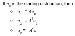
Once we have a trend identified and we know our starting distribution, we can predict future distributions. This obviously can have many power applications.
The Steady State
A major reason Markov matrices matter is that many systems approach steady states. The steady state Au = u →(A – I)u = u. This means u is an eigenvector with eigenvalue = 1. The steady state is a distribution that does not change after another application of the matrix.
Why Eigenvalues Matter
The eigenvalue of 1 gives the long term steady state, while other eigenvalues describe temporary parts of a system. If those eigenvalues have an absolute value of less than one, then their effects diminish over repeated matrix multiplications. That is why
Aku0 → u∞
Over time, the matrix system approaches a steady state.
Population Growth: Similar Matrix Idea, Different Meaning
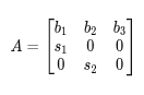
Population growth models use matrix powers, although they are not necessarily Markov matrices, as total population can increase or decrease. Here for example, we have a population divided into 3 age groups
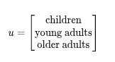
This population might include
- Birth rates
- Survival rates
- Aging into the next age group
- Death rates
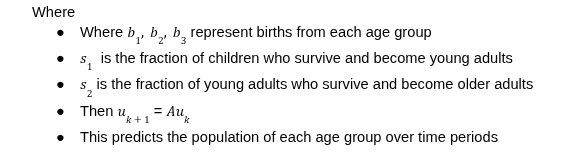
Take, for example:
Population Growth and Dominant Eigenvalues
For population matrices, the dominant eigenvalue is important. If it is greater than 1, the population grows, less than 1, it shrinks, or stays the same when the eigenvalue is 1. I found this interesting given the context of declining populations over much of the world – this is how we’re able to project populations.
Economics and the Consumption Matrix
A consumption matrix describes how much each industry consumes from other industries to produce one unit of output. For example, suppose an economy is composed of agriculture, manufacturing, and energy. A matrix entry aij tells us how much input is needed from industry i to produce one unit of output in industry j.
Product and Demand
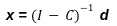
If x is the total production vector, and d is final demand, then part of the production is consumed internally by the economy. We can say internal consumption is Cx. As such, tota production must satisfy x = Cx + d. So, x – Cx = d → (I – C)x = d. We can then determine how much each industry must produce to satisfy final demand after accounting for inter-industry consumption. We can conclude that
Summary
Markov matrices, population matrices, and consumption matrices all show the same central idea:
- A matrix describes relationships between parts of a system, and linear algebra helps predict the system’s behavior.
- Markov matrices show how a distribution changes over time
- A population matrix shows how a population expands, shrinks, or stabilizes over time
- A consumption matrix shows how much production is needed to meet demand
There is lots to process in this dense section, but also much to ponder as I continue to see the application of Linear Algebra in the real world.