

Professor Leonard – Calculus 3 – 13.1: Introduction to Multivariable Functions (Domain, Sketching, Level Curves)
Thomas – 14.1 Functions of Several Variables
Multivariable Functions
Up to this point, calculus operations have involved a single variable. A function relates one or more input variables to a single output variable. In Calculus I and Calculus II, we studied functions of a single variable, such as f(x). Calculus is the study of how functions change, primarily through differentiation and integration.
I am writing this from the beautiful, seaside city of Vung Tau, Vietnam. It is hot in my room. Single Variable Calculus could be likened to examining how my room temperature changes as relative to the time change over a 24-hour period.
Multivariable Calculus, as the name implies, is Calculus with more than one variable. It is the study of the change of functions with multiple variables interacting to produce a given result at a given point. This could be the examination of how my room temperature changes as the time of day, humidity level, and wind conditions change.
Independent vs Dependent Variables
Every function is framed in terms of dependent and independent variables. Take f(x) = sin(x) for example. Here:
- x is the independent variable
- f(x) is the dependent variable (the output)
- sin(x) is the rule that defines the function
The heat in my room is the dependent variable, and the time of day the independent variable.
Likewise, for multivariable functions, f(x, y, z) is a dependent variable, while x, y, and z are independent variables. And the heat in my room depends on the independent time of day, the wind, and the humidity.
Graphing Multivariable Functions
A function of one variable is graphed in two dimensions. Think of the room temperature, with the independent variable time of day in the x-axis, and the temperature plotted along the y-axis at different times, or values of x.
Likewise, a function with two variables is graphed in three dimensions. The time of day and the humidity level are common independent variables (call these x and y), and my room temperature is still the dependent variable (now graphed along the z-axis). Since a function has a single output, each additional independent variable requires one additional graphing dimension. A function of one variable requires two dimensions, while a function of two variables requires three. Beyond that, visualization becomes impossible, even though the mathematics continues to work exactly the same way.
Domains of Multivariable Functions
The domain of a function is the set of all input values for which the function is defined. We often begin by assuming the domain is all real values of the input variables. We then identify constraints stemming from common mathematical restrictions, such as:
- Denominators can’t be equal to zero
- Denominators cannot equal zero
- Even roots (e.g., square roots) cannot have negative radicands
- Logarithm arguments must be positive
Sketching Domains
To sketch domains, we start with the boundary curves created by the aforementioned restrictions. We use a solid line if the boundary is included, and a dashed line if the boundary is not included. Then the remaining region is shaded where the function is defined. For example
- First sketch the boundary curves created by the restrictions.
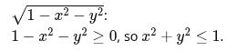
The domain is inside and on the circle. Whereas:
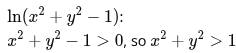
The domain is outside the circle with a dashed boundary line, indicating that the domain does not include the points along the circle.
Interior, Boundary, and Exterior Points
Points exist in reference to a given domain. If a set of points exist fully within the domain, they are interior points. Around an interior point, you could draw a small circle that stays within the domain.
Other points might lie on the edge of a domain. You could draw a small circle around such a point, and some of it will stay inside the domain, and some outside the domain. These are boundary points.
Finally, there are those points that exist completely outside of the domain. That small circle you draw around a point doesn’t even touch the domain boundary – it’s entirely outside of it. This is an exterior point.
Open vs. Closed Regions
An open region doesn’t include its boundary. Every point is safely inside the region. Conversely, a closed region is entirely outside the boundary. Some regions are neither open nor closed if they include only part of the boundary. For example:

Bounded vs. Unbounded Regions
A region is bounded if you can fit an entire region inside a circle. A region is unbounded if it stretches forever in at least one direction, so no circle can fully contain it. A bounded region is one that can be completely contained inside a circle of finite radius. An unbounded region extends infinitely far in at least one direction. For example:
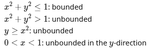
Ranges of Functions
The range of a function is the set of all output values the function can produce. Once the domain of a function has been established, we can determine the output values that are possible in regards to the domain constraints. WIth those values identified, we can then determine the range by analyzing the function and taking into account the domain-possible values. Some output values may be impossible because of the function’s behavior or because the domain excludes the inputs needed to produce them.
Level Curves
A level curve is the curve formed by intersecting the surface z = f(x, y) with a horizontal plane z = k. Equivalently, it is the set of all points (x, y) for which the function has the same value f(x, y) = k. A collection of level curves is called a contour map or contour plot. Level curves help us to visualize functions of three or more independent variables.
How to Sketch Level Curves
In order to sketch a level curve, first set the function equal to a constant, e.g. f(x, y) = k, then solve the resulting equation. With that equation established, identify the resulting family of curves (circles, ellipses, parabolas, hyperbolas, lines, etc.). Then sketch several curves using different values of k.
Reflections
This section really tripped me up. There was a large set of exercises where I’d have to find the a) domain, b) range, c) describe the level curve, d) find the boundary of the function, e) determine if the function was an open region/closed region/neither, and f) decide if the domain is bounded or unbounded. I always got some of a question right, but always bungled other parts of the question. Distinguishing bounded from boundaries, open or closed (or open and closed), and even seemingly simple questions about a range, were a thorn in my side. None of these, isolated on their own, are particularly confusing, but they obviously confused me. I think once the frustration set in, it made matters worse. So I spent days grinding through the questions.
Sketching is also a challenge for me. I’m weak when it comes to visualization. I don’t have an artistic bone in my body and struggle just to draw a sphere. So the level curve exercises were tough. When given a set of level curves and tasked with matching them to their functions and corresponding surfaces, I had relatively little problems. I understand what’s happening in the function and understand, more or less, what I see. But drawing, especially in 3D, is something else entirely. WolframAlpha (https://www.wolframalpha.com/) comes in incredibly handy in bypassing the tedium of sketching, as it does in so many other ways.