

Professor Leonard – Calculus 3
12.3: Arc Length/Parameterization, TNB (Frenet-Serret) Intro
Thomas – 13.3 ‘Arc Lengths in Space’
Arc Length
By now we’re familiar with parametric equations. They’re those very useful equations that describe a curve by expressing each coordinate as a function of a third variable, such as t (time). We use them because they let us model motion and curves that are difficult or impossible to describe with a single equation like y = f(x). We can calculate the length of a curve in two-dimensional space like this
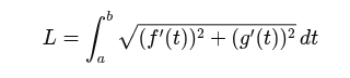
We can think of f’(t) as movement along the x-axis and g’(t) along the y-axis. You might notice the similarity with how we can calculate the length of a hypotenuse of a right triangle, i.e. as the square root of the sum of the squares of the base and height. At any rate, we can extend this concept into three-dimensional space by adding an additional function, call it h(t) if you like.
I’ll begin by building on a vector-valued function. Let’s call it:
r(t) = <x(t), y(t), z(t)>.
The derivative of of this function gives us the velocity (or tangent) vector
r’(t) = <x’(t), y’(t), z’(t)>
The magnitude of the velocity vector above gives us the speed:

The integral of the speed, i.e. the integral of the velocity vector’s magnitude, will tell us the length of a curve in space.
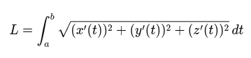
The compact way of saying this is
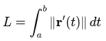
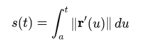
The way to think of this is that velocity r’(t) tells us how much distance and where (path of a curve in 3D space) over a unit of time, and the magnitude tells us the total distance traveled along a curve over t units of time. What’s more, when we don’t already have two fixed values, i.e. bounds, we can use the same formula to define our arc length function
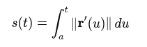
In this case, our upper bound becomes the variable t. We switch our integration variable to u so we don’t use t twice. In this way, s(t) indicates the distance traveled along a curve from the starting point up until t. This allows us to measure the position along a curve by actual distance traveled.
Reparameterizing by Arc Length
Instead of using t, we define
Where s represents the actual distance traveled along a curve. Let’s say we start at point 0, so s = 0 is the starting point.
- s = 5 means we’ve walked 5 units along the curve
- s =10 means we’ve walked 10 units along the curve
- s = n means we’ve walked n units along the curve
So the parameter now directly measures the distance along the curve. Why is this useful?
- The parameter becomes physical distance: Instead of some abstract t, the parameter literally tells us where we are along the curve.
- Many formulas simplify: Once parameterized, r(s) is easier to work with because ||dr/ds|| = 1. Why is that, might you ask? Because ds/ds = 1. So for every unit of parameter change, we travel exactly 1 unit along the curve. Motion occurs at a constant unit speed.
- The tangent vector becomes a unit tangent vector: Normally, r’(t) is a velocity vector whose magnitude changes. However, after reparameterization, r’(t) = dr/ds, which has a magnitude of 1. As such, it’s already the tangent vector T(s) = dr/ds – no normalization is required.
Reflections
- It’s cool to think that we could have some coiling, twisting path of a particle, or a growing noodle, and that we can determine its length with some ‘simple’ calculus.
- I was a little rusty with integration at first, having not practiced it in nearly six months. There were those “oh, I forgot that” moments. It was nice to practice integration again. Like riding a bike…
- Calculus makes sense! Even though it can be complex in terms of the concepts integrated into a problem, and although it’s unforgiving in its demand for attention to detail, in the end I just plug in pieces I’ve learned in the past and calculate an answer. Presto. It’s so refreshing after the abstract brain yoga a la Linear Algebra.